
Downward sloping of aggregate demand curve.
Explanation of Solution
The aggregate demand (AD) curve shows an inverse relation between price level and real
The aggregate demand curve slopes downward due to three reasons:
Real balance effect: A change in the price level produces the real balance effect. A rise in the price level, results in a decrease in the
Interest Rate Effect: Assuming the money supply in the economy to be fixed, rise in price level implies more money required for purchases and pay for inputs. So, an increase in money demanded would increase the price paid for it, that is. the interest rate. The rise in interest rate will increase the borrowing costs which decrease the investment expenditure. This will decrease the quantity of real output demanded, thus decreasing the aggregate demand.
Foreign Purchases Effect: It is one of the key reasons behind the sloping of the aggregate demand curve. When the domestic price level rises relative to foreign price levels, foreigners buy fewer domestic goods as it becomes more expensive and people (domestic) opt for more foreign goods. Therefore, the export of domestic goods decline and import of foreign goods rise. As a result, there will be a decline in the overall demand for our domestic output. Thus the aggregate quantity demanded of GDP will decline. This slopes the AD curve downwards.
The reasons for downward sloping of AD curve are different from the reason for downward sloping of demand curve of a single-product. Assuming, a constant money income, substitution effect can work on a single product, whereby dropping prices of a single product make it relatively cheaper product compared to the other products whose price have not been changed. Also, the consumer has become richer in real terms, as he could afford more of the product whose price has been declined. But with the AD curve, as all the prices are falling implies dropping of the price level, thus single product substitution effect is not applicable in AD curve. Also, while dealing with demand of a single product, money income is assumed to be fixed. But this assumption is not applicable in case of AD curve because with regard to the circular flow of the economy, lower prices indicate lower incomes. Thus a decline in the price level does not necessarily imply an increase in the nominal income of the economy as a whole since as prices are dropping, so are the receipts or revenue of the sellers.
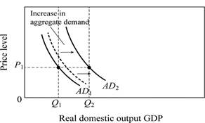
Figure-1
The multiplier effect acts on the initial change in spending to generate an even greater shift in the aggregate demand curve.
For instance, Figure 1 shows how multiplier effect works on an increase in income expenditure. The initial increase in spending is reflected by the broken line of AD curve, and then multiplier effect shift the AD curve from AD1 to AD2.
Concept Introduction:
Aggregate Demand: It refers to the total value of the goods and services available for purchase at a particular price in a given period of time.
Multiplier effect: Multiplier refers to the ratio of change in the real GDP to the change in initial consumption at constant price rate. Multiplier is positively related to the marginal propensity to consumer and negatively related with the marginal propensity to save.
Want to see more full solutions like this?
Chapter 12 Solutions
Macroeconomics

- The following graph shows a decrease in aggregate demand (AD) in a hypothetical country. Specifically, aggregate demand shifts to the left from AD1AD1 to AD2AD2, causing the quantity of output demanded to fall at all price levels. For example, at a price level of 140, output is now $200 billion, where previously it was $300 billion. The following table lists several determinants of aggregate demand. Complete the table by indicating the change in each determinant necessary to decrease aggregate demand. Change needed to decrease AD Wealth (increase/ decrease) Taxes (increase/ decrease) Expected rate of return on investment (increase/ decrease) Incomes in other countries (increase/ decrease)arrow_forwardThe figure given below represents the equilibrium real GDP and price level in the aggregate demand and aggregate supply model Figure 8.3 U.S. Price Level B O AD, toAD; O AD, to AD₂ O AD₂ to AD₁ O AS, to AS; AS; to AS₂ 100 200 300 400 AS3 AS₁ AD₂ 500 Real GDP (billions of dollars) AD AS₂ AD3 In Figure 8.3, which of the following shifts would result in stagflation (economic stagnation and inflation)?arrow_forwardSuppose that the price level is constant and that investment decreases sharply. How would you show this decrease in the aggregate expenditures model? What would be the outcome for real GDP? How would you show this fall in investment in the aggregate demand–aggregate supply model, assuming the economy is operating in what, in effect, is a horizontal section of the aggregate supply curve?arrow_forward
- In March 2020, as the Covid-19 recession hit the world, consumers became pessimistic about their future incomes. How did this increased pessimism affect the aggregate demand curve in the year 2020? Group of answer choices This will shift the aggregate demand curve to the right. This will move the economy down along a stationary aggregate demand curve. This will move the economy up along a stationary aggregate demand curve. This will shift the aggregate demand curve to the left.arrow_forwardUsing the three-point curved line drawing tool, show how the following event will impact the economy's short-run aggregate supply (AS) curve. Properly label this curve. 12- 11- Event: 10- High taxes and excessive regulation cause firms to reduce the quantity of their physical capital. 9- Note: Carefully follow the instructions above and only draw the required object. ASO 8- 4- 3- 2- 1- 0- 10 Aggregate output (income), Y Price level, Parrow_forwardeconomics Consider a goods market equilibrium (The aggregate expenditure model) in a closed economy a) Equationally and graphically (using the graph above) show (define) a goods market equilibrium b) Explain which factor changes the slope of the ZZ(or D, demand) curve and which factors shift the ZZ curve c) Suppose that marginal propensity to consume is equal to 0.8. Explain how much an increase in government spending 500 million of dollars raises real output and why output increases more than government spending?arrow_forward
- You will draw four separate Aggregate-Demand/Aggregate-Supply graphs. Each graph will have one curve shift. Be sure to label axis, curves, and equilibrium. Change colors to show the shift and label the new equilibrium. Draw an ADAS graph at equilibrium. Suppose the interest rates on loans on capital goods decrease. Which curve will shift? Draw the new equilibrium. Draw an ADAS graph at equilibrium. Suppose there is an decrease in government spending. Which curve will shift? Draw the new equilibrium. Draw an ADAS graph at equilibrium. Suppose the income of our trading partners increase. Which curve will shift? Draw the new equilibrium. Draw an ADAS graph at equilibrium. Suppose there is widespread concern that prices will continue to rise in the future. Which curve will shift? Draw the new equilibrium.arrow_forwardQuestion 1. Explain why the Aggregate Demand curve is downward sloping . 2. Explain why the Aggregate Supply curve is upward sloping . 3. What determines potential output Yf, and how can the economy exceed Yf in the short run? 4. Explain the Equilibrium condition of Aggregate Expenditure= output Y. How are inventory changes related to AE and Y? 5. Define the multiplier and the marginal propensities to consume (MPC) and save (MPS). What is the relationship between the MPC and the multiplier? 6. Compare and contrast the short run Keynesian and long run Neoclassical views of the aggregate supply and Phillips curves 7. For each the following economies, calculate equilibrium Y*, the multiplier, and the size of the recessionary or inflationary gap, if any. a. AE= 250 +.75 Y Yf= 1200 b. AE= 400+ .9 Y Yf= 3000 c. AE= 300 +. 8Y Yf=1500 d. AE= 300+ .67 Y Yf=1000arrow_forwardUsing a macroeconomics demand/supply analysis, where do you think current output is relative to what the economy is capable of producing? Look at recent trends in the data. What are the recent trends in the components of aggregate demand (consumption spending, investment spending, government purchases, and exports and imports?arrow_forward
- The following graph shows an aggregate demand curve (AD) illustrating the inverse relationship between the price level and the quantity of Real GDP in the United States. During World War II, the United States increased military spending. Show the effect of the following scenario on the aggregate demand curve by dragging the curve or moving the point to the appropriate position. Note: Tool tip: To move the curve, click and drag any part of the curve. The curve will snap into position, so if you try to move it and it snaps back to its original position, just try again and drag it a little farther. PRICE LEVEL Aggregate Demand I I " I 1 REAL GDP AD AD (?)arrow_forwardIn 2013, Prussia's aggregate demand curve was determined by the equation M + 1-4% A change in aggregate demand means that in 2014, Prussia's aggregate demand curve was determined by the equation Using this information, draw Prussia's old and new dynamic aggregate demand curves on the graph Which of the factors could have resulted in the change irn aggregate demand seen between 2013 and 2014? 13 AD 2013 an improvement in technology O an increase in imports O higher consumer confidence O a decrease in oil prices 12 AD 2014 10 8 5 4 3 2 4 -3 2 1 0 1 2 3 4 5 6 78 9 10 Real GDP growth ratearrow_forwardAssume the Potential GDP is $15 trillion dollars. Use the table below to answer the following questions. Assume all values represent trillions of dollars. Use the table to create two graphs: 1. aggregate expenditure model and 2. an aggregate supply aggregate demand model. Note that the equilibrium in the table above will determine your real GDP and your potential GDP should be plotted in both graphs. What type of macroeconomic equilibrium does this economy reflect? Note that the multiplier is 2 because this economy has imports. If Investment expenditures increase by $2.5, how much does GDP increase? Does the increase in investment expenditures from part C result in a full employment equilibrium? Why? Graphically show the effects from part C in our Aggregate Expenditure Model and Aggregate Supply-Aggregate Demand Model.arrow_forward

 Principles of Economics (12th Edition)EconomicsISBN:9780134078779Author:Karl E. Case, Ray C. Fair, Sharon E. OsterPublisher:PEARSON
 Engineering Economy (17th Edition)EconomicsISBN:9780134870069Author:William G. Sullivan, Elin M. Wicks, C. Patrick KoellingPublisher:PEARSON
 Principles of Economics (MindTap Course List)EconomicsISBN:9781305585126Author:N. Gregory MankiwPublisher:Cengage Learning
 Managerial Economics: A Problem Solving ApproachEconomicsISBN:9781337106665Author:Luke M. Froeb, Brian T. McCann, Michael R. Ward, Mike ShorPublisher:Cengage Learning
 Managerial Economics & Business Strategy (Mcgraw-...EconomicsISBN:9781259290619Author:Michael Baye, Jeff PrincePublisher:McGraw-Hill Education