Concept explainers
Videos
a.
To find:The regression equation for the data.
a.
Answer to Problem 21E
The regression equation for the data is
Explanation of Solution
Given information: The data is shown below.
| 31.3 | 50 | 19 | 4.0 | 37.4 | 60 | 30 | 5.0 | 24.0 | 60 | 24 | 4.0 | 51.0 | 80 | 34 | 7.5 |
| 56.9 | 90 | 38 | 8.0 | 43.3 | 60 | 26 | 7.0 | 36.2 | 50 | 21 | 7.0 | 34.3 | 60 | 22 | 2.5 |
| 43.1 | 70 | 28 | 6.5 | 36.3 | 70 | 25 | 7.5 | 26.5 | 50 | 17 | 2.0 | 31.5 | 60 | 24 | 5.0 |
| 41.5 | 70 | 25 | 5.5 | 38.4 | 70 | 31 | 5.5 | 47.1 | 80 | 34 | 8.5 | 33.2 | 60 | 23 | 4.0 |
| 39.0 | 60 | 26 | 6.5 | 41.5 | 60 | 27 | 7.5 | 38.1 | 70 | 27 | 5.5 | 39.2 | 60 | 29 | 6.5 |
| 40.9 | 70 | 29 | 5.0 | 36.l | 60 | 23 | 6.0 | 33.5 | 60 | 24 | 2.5 | 46.7 | 70 | 27 | 7.5 |
| 35.9 | 60 | 23 | 5.5 | 38.5 | 60 | 23 | 6.0 | 43.6 | 70 | 27 | 10.0 | 30.4 | 70 | 32 | 4.0 |
| 43.5 | 70 | 28 | 5.5 | 42.4 | 60 | 24 | 9.0 | 41.0 | 80 | 32 | 6.5 | 43.2 | 60 | 25 | 5.5 |
| 47.9 | 80 | 34 | 6.5 | 46.5 | 70 | 31 | 5.5 | 50.2 | 50 | 26 | 9.0 | 30.6 | 60 | 26 | 3.5 |
| 33.8 | 70 | 26 | 4.5 | 43.1 | 80 | 32 | 6.0 | 34.4 | 50 | 22 | 4.0 | 43.3 | 70 | 28 | 7.5 |
| 41.1 | 70 | 26 | 8.0 | 50.8 | 60 | 26 | 10.0 | 47.9 | 80 | 34 | 6.5 | 32.4 | 60 | 22 | 5.5 |
| 38.7 | 70 | 26 | 8.0 | 44.2 | 70 | 28 | 4.5 | 46.2 | 50 | 21 | 10.0 | 35.5 | 60 | 22 | 4.5 |
Calculation:
The MINITAB is shown below,
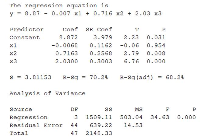
Figure-1
From Figure-1 it is clear that the regression equation is
b.
To find: The value of variable
b.
Answer to Problem 21E
The value of variable
Explanation of Solution
Given information: The data is shown below.
| 31.3 | 50 | 19 | 4.0 | 37.4 | 60 | 30 | 5.0 | 24.0 | 60 | 24 | 4.0 | 51.0 | 80 | 34 | 7.5 |
| 56.9 | 90 | 38 | 8.0 | 43.3 | 60 | 26 | 7.0 | 36.2 | 50 | 21 | 7.0 | 34.3 | 60 | 22 | 2.5 |
| 43.1 | 70 | 28 | 6.5 | 36.3 | 70 | 25 | 7.5 | 26.5 | 50 | 17 | 2.0 | 31.5 | 60 | 24 | 5.0 |
| 41.5 | 70 | 25 | 5.5 | 38.4 | 70 | 31 | 5.5 | 47.1 | 80 | 34 | 8.5 | 33.2 | 60 | 23 | 4.0 |
| 39.0 | 60 | 26 | 6.5 | 41.5 | 60 | 27 | 7.5 | 38.1 | 70 | 27 | 5.5 | 39.2 | 60 | 29 | 6.5 |
| 40.9 | 70 | 29 | 5.0 | 36.l | 60 | 23 | 6.0 | 33.5 | 60 | 24 | 2.5 | 46.7 | 70 | 27 | 7.5 |
| 35.9 | 60 | 23 | 5.5 | 38.5 | 60 | 23 | 6.0 | 43.6 | 70 | 27 | 10.0 | 30.4 | 70 | 32 | 4.0 |
| 43.5 | 70 | 28 | 5.5 | 42.4 | 60 | 24 | 9.0 | 41.0 | 80 | 32 | 6.5 | 43.2 | 60 | 25 | 5.5 |
| 47.9 | 80 | 34 | 6.5 | 46.5 | 70 | 31 | 5.5 | 50.2 | 50 | 26 | 9.0 | 30.6 | 60 | 26 | 3.5 |
| 33.8 | 70 | 26 | 4.5 | 43.1 | 80 | 32 | 6.0 | 34.4 | 50 | 22 | 4.0 | 43.3 | 70 | 28 | 7.5 |
| 41.1 | 70 | 26 | 8.0 | 50.8 | 60 | 26 | 10.0 | 47.9 | 80 | 34 | 6.5 | 32.4 | 60 | 22 | 5.5 |
| 38.7 | 70 | 26 | 8.0 | 44.2 | 70 | 28 | 4.5 | 46.2 | 50 | 21 | 10.0 | 35.5 | 60 | 22 | 4.5 |
Calculation:
From Figure-1 it is clear that the regression equation is
Substitute the values in above equation.
Thus, the value of variable
c.
To find: The confidence interval.
c.
Answer to Problem 21E
The confidence intervalis
Explanation of Solution
Given information: The data is shown below.
| 31.3 | 50 | 19 | 4.0 | 37.4 | 60 | 30 | 5.0 | 24.0 | 60 | 24 | 4.0 | 51.0 | 80 | 34 | 7.5 |
| 56.9 | 90 | 38 | 8.0 | 43.3 | 60 | 26 | 7.0 | 36.2 | 50 | 21 | 7.0 | 34.3 | 60 | 22 | 2.5 |
| 43.1 | 70 | 28 | 6.5 | 36.3 | 70 | 25 | 7.5 | 26.5 | 50 | 17 | 2.0 | 31.5 | 60 | 24 | 5.0 |
| 41.5 | 70 | 25 | 5.5 | 38.4 | 70 | 31 | 5.5 | 47.1 | 80 | 34 | 8.5 | 33.2 | 60 | 23 | 4.0 |
| 39.0 | 60 | 26 | 6.5 | 41.5 | 60 | 27 | 7.5 | 38.1 | 70 | 27 | 5.5 | 39.2 | 60 | 29 | 6.5 |
| 40.9 | 70 | 29 | 5.0 | 36.l | 60 | 23 | 6.0 | 33.5 | 60 | 24 | 2.5 | 46.7 | 70 | 27 | 7.5 |
| 35.9 | 60 | 23 | 5.5 | 38.5 | 60 | 23 | 6.0 | 43.6 | 70 | 27 | 10.0 | 30.4 | 70 | 32 | 4.0 |
| 43.5 | 70 | 28 | 5.5 | 42.4 | 60 | 24 | 9.0 | 41.0 | 80 | 32 | 6.5 | 43.2 | 60 | 25 | 5.5 |
| 47.9 | 80 | 34 | 6.5 | 46.5 | 70 | 31 | 5.5 | 50.2 | 50 | 26 | 9.0 | 30.6 | 60 | 26 | 3.5 |
| 33.8 | 70 | 26 | 4.5 | 43.1 | 80 | 32 | 6.0 | 34.4 | 50 | 22 | 4.0 | 43.3 | 70 | 28 | 7.5 |
| 41.1 | 70 | 26 | 8.0 | 50.8 | 60 | 26 | 10.0 | 47.9 | 80 | 34 | 6.5 | 32.4 | 60 | 22 | 5.5 |
| 38.7 | 70 | 26 | 8.0 | 44.2 | 70 | 28 | 4.5 | 46.2 | 50 | 21 | 10.0 | 35.5 | 60 | 22 | 4.5 |
Calculation:
The MINITAB output is shown below.
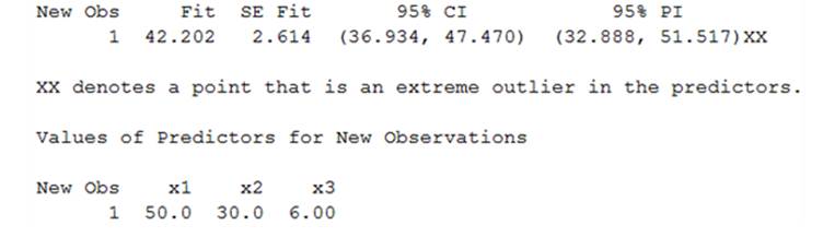
Figure-2
From Figure-2 it is clear that the confidence interval is
d.
To find: The prediction interval.
d.
Answer to Problem 21E
The prediction intervalis
Explanation of Solution
Given information: The data is shown below.
| 31.3 | 50 | 19 | 4.0 | 37.4 | 60 | 30 | 5.0 | 24.0 | 60 | 24 | 4.0 | 51.0 | 80 | 34 | 7.5 |
| 56.9 | 90 | 38 | 8.0 | 43.3 | 60 | 26 | 7.0 | 36.2 | 50 | 21 | 7.0 | 34.3 | 60 | 22 | 2.5 |
| 43.1 | 70 | 28 | 6.5 | 36.3 | 70 | 25 | 7.5 | 26.5 | 50 | 17 | 2.0 | 31.5 | 60 | 24 | 5.0 |
| 41.5 | 70 | 25 | 5.5 | 38.4 | 70 | 31 | 5.5 | 47.1 | 80 | 34 | 8.5 | 33.2 | 60 | 23 | 4.0 |
| 39.0 | 60 | 26 | 6.5 | 41.5 | 60 | 27 | 7.5 | 38.1 | 70 | 27 | 5.5 | 39.2 | 60 | 29 | 6.5 |
| 40.9 | 70 | 29 | 5.0 | 36.l | 60 | 23 | 6.0 | 33.5 | 60 | 24 | 2.5 | 46.7 | 70 | 27 | 7.5 |
| 35.9 | 60 | 23 | 5.5 | 38.5 | 60 | 23 | 6.0 | 43.6 | 70 | 27 | 10.0 | 30.4 | 70 | 32 | 4.0 |
| 43.5 | 70 | 28 | 5.5 | 42.4 | 60 | 24 | 9.0 | 41.0 | 80 | 32 | 6.5 | 43.2 | 60 | 25 | 5.5 |
| 47.9 | 80 | 34 | 6.5 | 46.5 | 70 | 31 | 5.5 | 50.2 | 50 | 26 | 9.0 | 30.6 | 60 | 26 | 3.5 |
| 33.8 | 70 | 26 | 4.5 | 43.1 | 80 | 32 | 6.0 | 34.4 | 50 | 22 | 4.0 | 43.3 | 70 | 28 | 7.5 |
| 41.1 | 70 | 26 | 8.0 | 50.8 | 60 | 26 | 10.0 | 47.9 | 80 | 34 | 6.5 | 32.4 | 60 | 22 | 5.5 |
| 38.7 | 70 | 26 | 8.0 | 44.2 | 70 | 28 | 4.5 | 46.2 | 50 | 21 | 10.0 | 35.5 | 60 | 22 | 4.5 |
Calculation:
From Figure-12 it is clear that the
e.
To find: The percentage of variation in variable
e.
Answer to Problem 21E
The percentage of variation in variable
Explanation of Solution
Given information: The data is shown below.
| 31.3 | 50 | 19 | 4.0 | 37.4 | 60 | 30 | 5.0 | 24.0 | 60 | 24 | 4.0 | 51.0 | 80 | 34 | 7.5 |
| 56.9 | 90 | 38 | 8.0 | 43.3 | 60 | 26 | 7.0 | 36.2 | 50 | 21 | 7.0 | 34.3 | 60 | 22 | 2.5 |
| 43.1 | 70 | 28 | 6.5 | 36.3 | 70 | 25 | 7.5 | 26.5 | 50 | 17 | 2.0 | 31.5 | 60 | 24 | 5.0 |
| 41.5 | 70 | 25 | 5.5 | 38.4 | 70 | 31 | 5.5 | 47.1 | 80 | 34 | 8.5 | 33.2 | 60 | 23 | 4.0 |
| 39.0 | 60 | 26 | 6.5 | 41.5 | 60 | 27 | 7.5 | 38.1 | 70 | 27 | 5.5 | 39.2 | 60 | 29 | 6.5 |
| 40.9 | 70 | 29 | 5.0 | 36.l | 60 | 23 | 6.0 | 33.5 | 60 | 24 | 2.5 | 46.7 | 70 | 27 | 7.5 |
| 35.9 | 60 | 23 | 5.5 | 38.5 | 60 | 23 | 6.0 | 43.6 | 70 | 27 | 10.0 | 30.4 | 70 | 32 | 4.0 |
| 43.5 | 70 | 28 | 5.5 | 42.4 | 60 | 24 | 9.0 | 41.0 | 80 | 32 | 6.5 | 43.2 | 60 | 25 | 5.5 |
| 47.9 | 80 | 34 | 6.5 | 46.5 | 70 | 31 | 5.5 | 50.2 | 50 | 26 | 9.0 | 30.6 | 60 | 26 | 3.5 |
| 33.8 | 70 | 26 | 4.5 | 43.1 | 80 | 32 | 6.0 | 34.4 | 50 | 22 | 4.0 | 43.3 | 70 | 28 | 7.5 |
| 41.1 | 70 | 26 | 8.0 | 50.8 | 60 | 26 | 10.0 | 47.9 | 80 | 34 | 6.5 | 32.4 | 60 | 22 | 5.5 |
| 38.7 | 70 | 26 | 8.0 | 44.2 | 70 | 28 | 4.5 | 46.2 | 50 | 21 | 10.0 | 35.5 | 60 | 22 | 4.5 |
Calculation:
From Figure-1 it is clear that the percentage of variation in variable
f.
To find:Whether the given model is useful for prediction.
f.
Answer to Problem 21E
The model is useful in prediction.
Explanation of Solution
Given information: The data is shown below.
| 31.3 | 50 | 19 | 4.0 | 37.4 | 60 | 30 | 5.0 | 24.0 | 60 | 24 | 4.0 | 51.0 | 80 | 34 | 7.5 |
| 56.9 | 90 | 38 | 8.0 | 43.3 | 60 | 26 | 7.0 | 36.2 | 50 | 21 | 7.0 | 34.3 | 60 | 22 | 2.5 |
| 43.1 | 70 | 28 | 6.5 | 36.3 | 70 | 25 | 7.5 | 26.5 | 50 | 17 | 2.0 | 31.5 | 60 | 24 | 5.0 |
| 41.5 | 70 | 25 | 5.5 | 38.4 | 70 | 31 | 5.5 | 47.1 | 80 | 34 | 8.5 | 33.2 | 60 | 23 | 4.0 |
| 39.0 | 60 | 26 | 6.5 | 41.5 | 60 | 27 | 7.5 | 38.1 | 70 | 27 | 5.5 | 39.2 | 60 | 29 | 6.5 |
| 40.9 | 70 | 29 | 5.0 | 36.l | 60 | 23 | 6.0 | 33.5 | 60 | 24 | 2.5 | 46.7 | 70 | 27 | 7.5 |
| 35.9 | 60 | 23 | 5.5 | 38.5 | 60 | 23 | 6.0 | 43.6 | 70 | 27 | 10.0 | 30.4 | 70 | 32 | 4.0 |
| 43.5 | 70 | 28 | 5.5 | 42.4 | 60 | 24 | 9.0 | 41.0 | 80 | 32 | 6.5 | 43.2 | 60 | 25 | 5.5 |
| 47.9 | 80 | 34 | 6.5 | 46.5 | 70 | 31 | 5.5 | 50.2 | 50 | 26 | 9.0 | 30.6 | 60 | 26 | 3.5 |
| 33.8 | 70 | 26 | 4.5 | 43.1 | 80 | 32 | 6.0 | 34.4 | 50 | 22 | 4.0 | 43.3 | 70 | 28 | 7.5 |
| 41.1 | 70 | 26 | 8.0 | 50.8 | 60 | 26 | 10.0 | 47.9 | 80 | 34 | 6.5 | 32.4 | 60 | 22 | 5.5 |
| 38.7 | 70 | 26 | 8.0 | 44.2 | 70 | 28 | 4.5 | 46.2 | 50 | 21 | 10.0 | 35.5 | 60 | 22 | 4.5 |
Calculation:
The null hypothesis is, the model is not useful for prediction and the alternative hypothesis is, the model is useful in prediction.
From Figure-1 it is clear that the p value is less than the level of significance of
Hence, the null hypothesis is rejected.
Thus, the model is useful in prediction.
g.
To explain:The test for the hypothesis
g.
Explanation of Solution
Given information: The data is shown below.
| 31.3 | 50 | 19 | 4.0 | 37.4 | 60 | 30 | 5.0 | 24.0 | 60 | 24 | 4.0 | 51.0 | 80 | 34 | 7.5 |
| 56.9 | 90 | 38 | 8.0 | 43.3 | 60 | 26 | 7.0 | 36.2 | 50 | 21 | 7.0 | 34.3 | 60 | 22 | 2.5 |
| 43.1 | 70 | 28 | 6.5 | 36.3 | 70 | 25 | 7.5 | 26.5 | 50 | 17 | 2.0 | 31.5 | 60 | 24 | 5.0 |
| 41.5 | 70 | 25 | 5.5 | 38.4 | 70 | 31 | 5.5 | 47.1 | 80 | 34 | 8.5 | 33.2 | 60 | 23 | 4.0 |
| 39.0 | 60 | 26 | 6.5 | 41.5 | 60 | 27 | 7.5 | 38.1 | 70 | 27 | 5.5 | 39.2 | 60 | 29 | 6.5 |
| 40.9 | 70 | 29 | 5.0 | 36.l | 60 | 23 | 6.0 | 33.5 | 60 | 24 | 2.5 | 46.7 | 70 | 27 | 7.5 |
| 35.9 | 60 | 23 | 5.5 | 38.5 | 60 | 23 | 6.0 | 43.6 | 70 | 27 | 10.0 | 30.4 | 70 | 32 | 4.0 |
| 43.5 | 70 | 28 | 5.5 | 42.4 | 60 | 24 | 9.0 | 41.0 | 80 | 32 | 6.5 | 43.2 | 60 | 25 | 5.5 |
| 47.9 | 80 | 34 | 6.5 | 46.5 | 70 | 31 | 5.5 | 50.2 | 50 | 26 | 9.0 | 30.6 | 60 | 26 | 3.5 |
| 33.8 | 70 | 26 | 4.5 | 43.1 | 80 | 32 | 6.0 | 34.4 | 50 | 22 | 4.0 | 43.3 | 70 | 28 | 7.5 |
| 41.1 | 70 | 26 | 8.0 | 50.8 | 60 | 26 | 10.0 | 47.9 | 80 | 34 | 6.5 | 32.4 | 60 | 22 | 5.5 |
| 38.7 | 70 | 26 | 8.0 | 44.2 | 70 | 28 | 4.5 | 46.2 | 50 | 21 | 10.0 | 35.5 | 60 | 22 | 4.5 |
The null hypothesis is, there is no relationship between
For the variable
From Figure-1 it is clear that the p value is
Hence, the null hypothesis is not rejected.
Thus, there is no linear relationship between
For the variable
From Figure-1 it is clear that the p value is
Hence, the null hypothesis is rejected.
Thus, there is alinear relationship between
For the variable
From Figure-1 it is clear that the p value is
Hence, the null hypothesis is rejected.
Thus, there is a linear relationship between
Want to see more full solutions like this?
Chapter 13 Solutions
Elementary Statistics ( 3rd International Edition ) Isbn:9781260092561


- If your graphing calculator is capable of computing a least-squares sinusoidal regression model, use it to find a second model for the data. Graph this new equation along with your first model. How do they compare?arrow_forwardDoes Table 2 represent a linear function? If so, finda linear equation that models the data.arrow_forwardA 10-year study conducted by the American Heart Association provided data on how age, blood pressure, and smoking related to the risk of strokes. The data file “Stroke.xslx” includes a portion of the data from the study. The variable “Risk of Stroke” is measured as the percentage of risk (proportion times 100) that a person will have a stroke over the next 10-year period. Regression Analysis As Image: 1) Based on the simple regression analysis output, write the estimated regression equation. 2) What is the correlation coefficient between Risk of Stroke and Age? How do you find iarrow_forward
- Calculate slope and intercept of the regression line.arrow_forward(15 Pt) 10. Jamie made the plot for her car showing the miles she drove on nine trips and the gas she uses. Gas Usage Distance Driven (Miles) 1 500 450 400 350 300 250 200 150 100 50 0 0 2 4 6 Gas Used (Gallons) 8 y = 35.475x + 32.893 10 ^ The equation for the regression line is y=32.893+35.475x. Jamie's car has 2 gallons of gas left. Estimate how far she can drive before running out of gas. Good Luck! 12arrow_forward
 Glencoe Algebra 1, Student Edition, 9780079039897...AlgebraISBN:9780079039897Author:CarterPublisher:McGraw Hill
 Trigonometry (MindTap Course List)TrigonometryISBN:9781305652224Author:Charles P. McKeague, Mark D. TurnerPublisher:Cengage Learning
 Algebra: Structure And Method, Book 1AlgebraISBN:9780395977224Author:Richard G. Brown, Mary P. Dolciani, Robert H. Sorgenfrey, William L. ColePublisher:McDougal Littell
 Algebra & Trigonometry with Analytic GeometryAlgebraISBN:9781133382119Author:SwokowskiPublisher:Cengage