Concept explainers
Videos
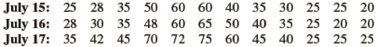
Air pollution control specialists in southern California monitor the amount of ozone, carbon dioxide, and nitrogen dioxide in the air on an hourly basis. The hourly time series data exhibit seasonality, with the levels of pollutants showing patterns that vary over the hours in the day. On July 15, 16, and 17, the following levels of nitrogen dioxide were observed for the 12 hours from 6:00 A.M. to 6:00 P.M.
- a. Construct a time series plot. What type of pattern exists in the data?
- b. Use the following dummy variables to develop an estimated regression equation to account for the seasonal effects in the data.
Hour1 = 1 if the reading was made between 6:00 A.M. and 7:00 A.M.; 0 otherwise
Hour2 = 1 if if the reading was made between 7:00 A.M. and 8:00 A.M.; 0 otherwise
.
.
.
Hour11 = 1 if the reading was made between 4:00 P.M. and 5:00 P.M., 0 otherwise.
Note that when the values of the 11 dummy variables are equal to 0, the observation corresponds to the 5:00 P.M. to 6:00 P.M. hour.
- c. Using the estimated regression equation developed in part (a), compute estimates of the levels of nitrogen dioxide for July 18.
- d. Let t = 1 to refer to the observation in hour 1 on July 15; t = 2 to refer to the observation in hour 2 of July 15; … and t = 36 to refer to the observation in hour 12 of July 17. Using the dummy variables defined in part (b) and t, develop an estimated regression equation to account for seasonal effects and any linear trend in the time series. Based upon the seasonal effects in the data and linear trend, compute estimates of the levels of nitrogen dioxide for July 18.
Want to see the full answer?
Check out a sample textbook solution
Chapter 17 Solutions
Modern Business Statistics with Microsoft Office Excel (with XLSTAT Education Edition Printed Access Card) (MindTap Course List)


- Find the mean hourly cost when the cell phone described above is used for 240 minutes.arrow_forwardAnswer C & D. Use the given data as reference.arrow_forwardA teacher asks their students whether they studied for a quiz, then scores the quiz. A relative frequency table displays some of the information they collectedarrow_forward
- Aypee kept track of the number of hours he studied each day for a 3-hour week period. The following observations (in hours) were recorded:Week 1: 1.5, 1.0, 0, 1.4, 0, 2.5, 0.8Week 2: 0.5, 2.0, 0.6, 0, 2.5, 1.8, 3.8Week 3: 0, 1.4, 2.2, 1.4, 0, 3.2, 0 Required: What is the modal number of hours studied per day? What is the median number of hours studied per day? What is the mean number of hours studied per dayarrow_forwardFind the relative frequency for the table shown below.arrow_forwardThe normal daily temperature for Honolulu, Hawaii are given by the following table. Find the equation that will model this data.arrow_forward
 Glencoe Algebra 1, Student Edition, 9780079039897...AlgebraISBN:9780079039897Author:CarterPublisher:McGraw Hill
 College Algebra (MindTap Course List)AlgebraISBN:9781305652231Author:R. David Gustafson, Jeff HughesPublisher:Cengage Learning
 Holt Mcdougal Larson Pre-algebra: Student Edition...AlgebraISBN:9780547587776Author:HOLT MCDOUGALPublisher:HOLT MCDOUGAL
 Functions and Change: A Modeling Approach to Coll...AlgebraISBN:9781337111348Author:Bruce Crauder, Benny Evans, Alan NoellPublisher:Cengage Learning